All office white-collar workers must use tools such as online forms (such as Google Sheets) for collaborative office work. Today, many platforms will introduce to you the skills and methods commonly used by Google Sheets to improve work efficiency. Get twice the result with half the effort at work.
Functions are a key component of spreadsheet applications such as Google Sheets. However, they can be overwhelming if you rarely use them, or if you’re just getting started. For the most basic things you’ll want to do, here are a couple of simple Google Sheets functions.
1. Addend: SUM
When working with numbers, it doesn’t get much more basic than adding them. Using this SUMfunction , you can add multiple numbers, add numbers in a cell, or use combinations.
The function’s syntax is SUM(value1, value2,...)required value1and value2optional .
To add the numbers 10, 20 and 30, you can use the following formula:
=SUM(10,20,30)
To add the numbers in cells A1 to A5, you can use the following formula:
=SUM(A1:A5)
The syntax for Google Sheets functions is value1required and value2optional.
To find the average of the numbers 10, 20 and 30, you can use the following formula:
=AVERAGE(10,20,30)
To find the average of the numbers in cells A1 to A5, use this formula:
=AVERAGE(A1:A5)
Tip: You can also view basic calculations without formulas in Google Sheets.
3. Count cells with numbers: COUNT
If you’ve ever had to count cells, you’ll love this COUNTfeature . With it, you can count how many cells in a range contain numbers.
The function’s syntax is COUNT(value1, value2,...)required value1and value2optional .
To count cells A1 to A5, you can use the following formula:
=COUNT(A1:A5)
To calculate cells A1 to A5 and D1 to D5, use the following formula:
=COUNT(A1:A5,D1:D5)
You can also use Google Sheets to calculate eligible data. COUNTIF
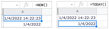
4. Enter the current date and time: now and today
If you want to see the current date and time every time you open Google Sheets, you can use NOWthe or TODAYfunction. NOWShows the date and time, while TODAYjust shows the current date.
The syntax for each is NOW()and TODAY()has no required parameters. Simply enter one or both of the following into the worksheet to display the date and time or just the date.
NOW() TODAY()
If you’d like your dates to appear in a certain format, you can set a default date format in Google Sheets.
5. Remove non-printable characters: CLEAN
When you import data into a worksheet from another location, the data may contain nonprintable or ASCII characters, such as backspaces and carriage returns. This CLEANfunction removes visible and invisible characters.
The syntax is consistent CLEAN(text)with the desired text.
To remove non-printable characters from the text in cell A1, you can use the following formula:
=CLEAN(A1)
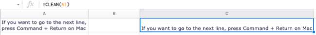
Note: Since the function removes characters you can’t see as well as characters you can see, you may not notice the difference in the resulting cells.
6. Remove blanks: TRIM
Another useful feature for organizing worksheets is TRIMthe function . Just like in Microsoft Excel, this function removes spaces in cells.
Syntax is where TRIM(text)text can represent a cell reference or actual text.
To remove the blanks in cell A1, you would use the following formula:
=TRIM(A1)
To remove spaces from “Remove Extra Space”, use the following formula:
=TRIM(“Remove extra spaces”)
7. Combining text or values: CONCATENATE and CONCAT
To combine strings, text or values, you can use CONCATENATEthe and CONCATfunction. The main difference between the two is that CONCATENATEprovides greater flexibility. For example, you can combine words and insert spaces between them.
The syntax for each parameter is CONCATENATE(string1, string2,...), and CONCAT(value1, value2)all parameters except string2are required.
To combine the values in cells A1 and B1, you can use the following formula:
=CONCATENATE(A1,B1)
To combine the words “How”, “To” and “Geek” with a space, you can use the following formula:
=CONCATENATE(“how to”, “”, “to”, “”, “geek”)
To combine the values 3 and 5, you can use the following formula:
=CONCAT(3,5)
For more details on these two features, check out our approach to connecting data in Google Sheets.
8. Insert an image in a cell: IMAGE
While Google Sheets provides the ability to insert images into cells, this IMAGEfeature gives you additional options to resize it or set a custom height and width in pixels.
The function’s syntax is IMAGE(url, mode, height, width)URL is required, other parameters are optional.
To insert an image with a URL as is, you would use the following formula:
=IMAGE(“https://abc.com/wp-content/uploads/2019/11/How-To_Geek_Logo.png”)
To insert the same image resized with a custom height and width, use the following formula:
=IMAGE(“https://abc.com/wp-content/uploads/2019/11/How-To_Geek_Logo.png”,4,50,200)
In this 4formula is a mode that allows custom image sizes of 50 x 200 pixels.
Note: You cannot use SVG graphics or URLs for images in Google Drive.
For more help on how to resize images using this feature, visit the Docs Editors help page for the IMAGE feature.
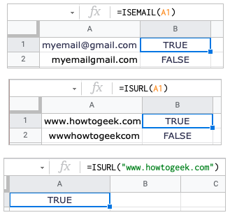
9. Verify email address or link: ISEMAIL and ISURL
Whether you’re importing or entering data in Google Sheets, you may want to verify that it’s as expected. Using ISEMAILand ISURL, you can ensure that the data is either an email address or a valid URL.
Each syntax is ISEMAIL(value)and ISURL(value)where you can use cell references or text. Validation results are displayed as TRUE or FALSE.
To check the email address in cell A1, you can use the following formula:
=ISEMAIL(A1)
To check the URL in cell A1, use the following formula:
=ISURL(A1)
To use text in a formula for an email address or URL, simply enclose it in quotation marks, like this:
=ISURL(“www.henduohao.com”)
Recommended purchase: Google account purchase Google account wholesale